Using Linear Algebra To Predict A Non-Linear Pendulum

An excruciating explainer into Koopman Operator methods for non-linear systems.

Biological systems are non-linear. Non-linear systems are hard to reason about. But Koopman operators (Koopman 1931) are a clever method of attack that converts non-linear systems into linear ones.

The benefit is that we can use the familiar tools of linear algebra to predict future behaviour. Linear systems are much easier to solve with computers than non linear ones, and we have tools like stability analysis to judge their qualitative properties.

The drawback is that we need to add (potentially infinitely more) variables to the system. But in modern times, this is less of an issue since we have better processors.

In this post, I’ll go into excruciating detail about how we can predict the non-linear motion of a simple pendulum using Koopman’s techniques. Given the amount of computing power we have now, we should probably be taking a fresh look at these kinds of methods.

Here is the result, if you can’t wait:

I hope to renew some optimism that we can look at some of these techniques for non-linear systems in biology, like the Lotka-Volterra equations, or chemical networks.

This is technical piece, but if you have a basic math background please follow along, its not too hard! The rest of this post is an explainer of the much more obtuse paper Koopman, B. O. (1931). “Hamiltonian systems and transformation in Hilbert space.”

---

An example of a simple non-linear system is the damped pendulum. This is a mass m attached to a rigid rod of length L, swinging under gravity. The system is fully described by two variables - its angle, and its angular velocity.

\(\begin{align} \theta(t) &\text{ : angle from vertical (radians) } \\ \omega(t) &= \dot{\theta}(t) \text{ : angular velocity (rad/s) } \end{align}\)

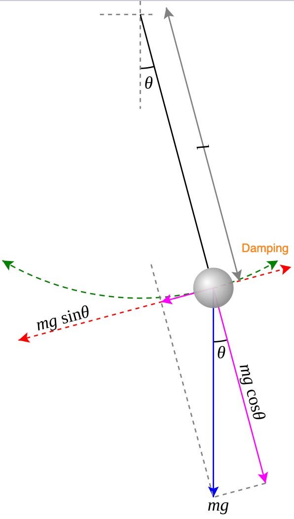
The gravitational force perpendicular to the rod creates a force of mg sin(θ). This creates a torque: τ_g = -mgL sin(θ). We also having a damping factor, due to air resistance, that is proportional to the speed of the pendulum. This is a force with strength -γ ω, and creates damping torque: τ_d = -γ L ω.

And so, the damped pendulum is described by the system of equations

\(\begin{align} \frac{d\theta}{dt} &= \omega \\ \frac{d\omega}{dt} &= -\frac{g}{L}\sin(\theta) - \gamma \omega \end{align} \)

where g is gravitational acceleration and γ is the damping coefficient.

---

The Koopman Transformation Trick.

sin is a non linear function of the variable θ, and so the sin(θ) term makes this system a non-linear differential equation.

To get over this, one naive thing we can do is to label the sin(θ) term as its own variable, and see what happens. Let’s set

\(s = \sin(\theta)\)

Now our system is

\(\begin{align} \frac{d\theta}{dt} &= \omega \\ \frac{d\omega}{dt} &= -\frac{g}{L}s - \gamma \omega \end{align}\)

This makes the first two equations linear in the variables involved. But, we are not allowed to just stop here. Doing this trick is not without a cost. Since s evolves as well, we also need to add s to our system whole sytem of equations. This gives us a system of three equations instead of two.

\(\begin{align} \frac{d\theta}{dt} &= \omega \text{, which is linear. } \\ \frac{d\omega}{dt} &= -\frac{g}{L}s - \gamma \omega \text{, which is linear. } \\ \frac{ds}{dt} &= \frac{d}{dt}\sin(\theta) = \cos(\theta) \cdot \frac{d\theta}{dt} = \cos(\theta) \cdot \omega \end{align}\)

We now have three equations, but the equation for s is not linear since it has a cos(θ) term, and is also multiplied by a state variable ω. Let’s play dumb and replace this with a variable c as well, and continue the procedure.

\(\begin{align} \frac{d\theta}{dt} &= \omega \\ \frac{d\omega}{dt} &= -\frac{g}{L}s - \gamma \omega \\ \frac{ds}{dt} &= c \cdot \omega \end{align}\)

We still need to add the evolution of c, so we differentiate it again.

\(\frac{dc}{dt} = \frac{d}{dt}\cos(\theta) = -\sin(\theta) \cdot \frac{d\theta}{dt} = -s \cdot \omega \)

Now we have a system with 4 variables: (θ, ω, s, c)

\(\begin{align} \frac{d\theta}{dt} &= \omega \\ \frac{d\omega}{dt} &= -\frac{g}{L}s - \gamma \omega \\ \frac{ds}{dt} &= c \cdot \omega \\ \frac{dc}{dt} &= -s \cdot \omega \end{align}\)

Even though we’ve got rid of the sin and cos terms, the last two equations still have products like c · ω and s · ω. This still makes them non-linear, since they are product of two variables.

We can still push ahead though, and add even more variables. Before that, instead of thinking of s and c as “new state variables,” let’s think of them as observables and give them new names.

- ψ₁(θ, ω) = θ (the angle)

- ψ₂(θ, ω) = ω (the angular velocity)

- ψ₃(θ, ω) = sin(θ) (the sine of the angle)

- ψ₄(θ, ω) = cos(θ) (the cosine of the angle)

When the state (θ, ω) evolves according to the pendulum equations, the other observables evolve as:

\(\begin{align} \frac{d\psi_1}{dt} &= \frac{d\theta}{dt} = \omega = \psi_2 \\ \frac{d\psi_2}{dt} &= \frac{d\omega}{dt} = -\frac{g}{L}\sin(\theta) - \gamma \omega = -\frac{g}{L}\psi_3 - \gamma \psi_2 \\ \frac{d\psi_3}{dt} &= \frac{d}{dt}\sin(\theta) = \cos(\theta) \cdot \omega = \psi_4 \cdot \psi_2 \\ \frac{d\psi_4}{dt} &= \frac{d}{dt}\cos(\theta) = -\sin(\theta) \cdot \omega = -\psi_3 \cdot \psi_2 \end{align}\)

Following the procedure before, since ψ₄ · ψ₂ and ψ₃ · ψ₂ aren’t in our observable space yet, we add them:

- ψ₅(θ, ω) = sin(θ) · ω = ψ₃ · ψ₂

- ψ₆(θ, ω) = cos(θ) · ω = ψ₄ · ψ₂

And so now we have

\(\begin{align} \frac{d\psi_3}{dt} &= \psi_6 \\ \frac{d\psi_4}{dt} &= -\psi_5 \end{align}\)

But we need to know how ψ₅ and ψ₆ evolve, so we add even more equations

\( \begin{align} \frac{d\psi_5}{dt} &= \frac{d}{dt}(\sin(\theta) \cdot \omega) = \cos(\theta) \cdot \omega^2 + \sin(\theta) \cdot \frac{d\omega}{dt} \\ &= \psi_4 \cdot \omega^2 + \psi_3 \cdot \left(-\frac{g}{L}\psi_3 - \gamma \psi_2\right) \end{align}\)

And so we need ω² as another observable! But by now, you have got the point. As we keep adding observables to “close” the system (make all derivatives expressible in terms of a linear combination of existing observables), we’re building up an infinite-dimensional space of new variables. Sometimes, the procedure ends. But most of the time, the process goes on forever.

In the case of the damped pendulum, we end up with an observable space like

\(\boldsymbol{\psi} = (\theta, \omega, \sin(\theta), \cos(\theta), \theta^2, \omega^2, \theta\omega, \sin(2\theta), \cos(2\theta), \ldots)\)

Where we’ve transformed the non linear system into a linear one

\(\frac{d}{dt}\boldsymbol{\psi} = \mathbf{K} \boldsymbol{\psi} \)

where K is a linear operator - the Koopman operator.

So what does K look like. Based on our evolution equations, let’s see the structure. For the first 4 observables, we have

\(\frac{d}{dt}\begin{pmatrix} \psi_1 \\ \psi_2 \\ \psi_3 \\ \psi_4 \end{pmatrix} = \begin{pmatrix} \frac{d\psi_1}{dt} \\ \frac{d\psi_2}{dt} \\ \frac{d\psi_3}{dt} \\ \frac{d\psi_4}{dt} \end{pmatrix} = \begin{pmatrix} \psi_2 \\ -\frac{g}{L}\psi_3 - \gamma \psi_2 \\ \psi_4 \cdot \psi_2 \\ -\psi_3 \cdot \psi_2 \end{pmatrix}\)

But ψ₄ · ψ₂ and -ψ₃ · ψ₂ aren’t linear combinations yet! We need to add ψ₅ = ψ₄ · ψ₂ and ψ₆ = ψ₃ · ψ₂. Then:

\(\frac{d}{dt}\begin{pmatrix} \psi_1 \\ \psi_2 \\ \psi_3 \\ \psi_4 \\ \psi_5 \\ \psi_6 \end{pmatrix} = \begin{pmatrix} \psi_2 \\ -\frac{g}{L}\psi_3 - \gamma \psi_2 \\ \psi_6 \\ -\psi_5 \\ \text{(needs more observables)} \\ \text{(needs more observables)} \end{pmatrix}\)

So the **partial** K matrix (for the first 6 observables) looks like:

\(\mathbf{K}_{6 \times 6} = \begin{pmatrix} 0 & 1 & 0 & 0 & 0 & 0 \\ 0 & -\gamma & -\frac{g}{L} & 0 & 0 & 0 \\ 0 & 0 & 0 & 0 & 0 & 1 \\ 0 & 0 & 0 & 0 & -1 & 0 \\ ? & ? & ? & ? & ? & ? \\ ? & ? & ? & ? & ? & ? \end{pmatrix} \)

The `?` entries show that dψ₅/dt and dψ₆/dt require more observables (like ω², sin²(θ), etc.) to be expressed as linear combinations.

---

On To Prediction!

Now that we have a basis set of observables, we can do some pretty interesting things. One is ‘learning’ the motion of the pendulum by using these observables as a basis! The following method is called the ‘extended dynamic mode decomposition approach’.

The intuition is to add the observables above, to closely approximate the non-linear system, and find a matrix that gives us the next time step.

\(\boldsymbol{\psi}(t +\Delta t) = \mathbf{K} \boldsymbol{\psi}(t)\)

First, we measure the system to get states x(t₁), x(t₂), …, x(t_M). For a pendulum, these are [θ(t_i), ω(t_i)] pairs

Suppose we have collected M=5 time points with states, from recording it wth a camera, or doing a simulation.

\(\begin{align} \mathbf{x}(t_1) &= [\theta(t_1), \omega(t_1)] = [0.5, 0.2] \\ \mathbf{x}(t_2) &= [\theta(t_2), \omega(t_2)] = [0.6, 0.15] \\ \mathbf{x}(t_3) &= [\theta(t_3), \omega(t_3)] = [0.65, 0.1] \\ \mathbf{x}(t_4) &= [\theta(t_4), \omega(t_4)] = [0.7, 0.05] \\ \mathbf{x}(t_5) &= [\theta(t_5), \omega(t_5)] = [0.72, 0.0] \end{align}\)

We then choose N=6 observables, from the observable space that we chose in the previous example.

\(\begin{align} \psi_1(\mathbf{x}) &= \theta \\ \psi_2(\mathbf{x}) &= \omega \\ \psi_3(\mathbf{x}) &= \sin(\theta) \\ \psi_4(\mathbf{x}) &= \cos(\theta) \\ \psi_5(\mathbf{x}) &= \theta^2 \\ \psi_6(\mathbf{x}) &= \omega^2 \end{align}\)

The idea is to build a matrix that ‘predicts’ then next time step. So we select the first 4 time steps to build Matrix X (observables at times t₁ to t₄):

Each column is ψ(x(t_i)):

\(\mathbf{X} = \begin{pmatrix} \theta(t_1) & \theta(t_2) & \theta(t_3) & \theta(t_4) \\ \omega(t_1) & \omega(t_2) & \omega(t_3) & \omega(t_4) \\ \sin(\theta(t_1)) & \sin(\theta(t_2)) & \sin(\theta(t_3)) & \sin(\theta(t_4)) \\ \cos(\theta(t_1)) & \cos(\theta(t_2)) & \cos(\theta(t_3)) & \cos(\theta(t_4)) \\ \theta(t_1)^2 & \theta(t_2)^2 & \theta(t_3)^2 & \theta(t_4)^2 \\ \omega(t_1)^2 & \omega(t_2)^2 & \omega(t_3)^2 & \omega(t_4)^2 \end{pmatrix} \)

Substituting our example values:

\(\mathbf{X} = \begin{pmatrix} 0.5 & 0.6 & 0.65 & 0.7 \\ 0.2 & 0.15 & 0.1 & 0.05 \\ \sin(0.5) & \sin(0.6) & \sin(0.65) & \sin(0.7) \\ \cos(0.5) & \cos(0.6) & \cos(0.65) & \cos(0.7) \\ 0.5^2 & 0.6^2 & 0.65^2 & 0.7^2 \\ 0.2^2 & 0.15^2 & 0.1^2 & 0.05^2 \end{pmatrix}\)

The we shift time by one unit, to build Matrix Y (observables at times t₂ to t₅). Each column is ψ(x(t_{i+1})):

\( \mathbf{Y} = \begin{pmatrix} \theta(t_2) & \theta(t_3) & \theta(t_4) & \theta(t_5) \\ \omega(t_2) & \omega(t_3) & \omega(t_4) & \omega(t_5) \\ \sin(\theta(t_2)) & \sin(\theta(t_3)) & \sin(\theta(t_4)) & \sin(\theta(t_5)) \\ \cos(\theta(t_2)) & \cos(\theta(t_3)) & \cos(\theta(t_4)) & \cos(\theta(t_5)) \\ \theta(t_2)^2 & \theta(t_3)^2 & \theta(t_4)^2 & \theta(t_5)^2 \\ \omega(t_2)^2 & \omega(t_3)^2 & \omega(t_4)^2 & \omega(t_5)^2 \end{pmatrix}\)

Substituting our example values:

\(\mathbf{Y} = \begin{pmatrix} 0.6 & 0.65 & 0.7 & 0.72 \\ 0.15 & 0.1 & 0.05 & 0.0 \\ \sin(0.6) & \sin(0.65) & \sin(0.7) & \sin(0.72) \\ \cos(0.6) & \cos(0.65) & \cos(0.7) & \cos(0.72) \\ 0.6^2 & 0.65^2 & 0.7^2 & 0.72^2 \\ 0.15^2 & 0.1^2 & 0.05^2 & 0.0^2 \end{pmatrix}\)

And now we solve for the matrix that gives us Y from X. From data, we have Y = K X. And we solve for K using least squares: K = Y X⁺ where X⁺ is the pseudoinverse. This gives us the finite-dimensional approximation K_N (an N × N matrix)

The learned Koopman operator K is a 6 × 6 matrix, and we can use this to predict evolution.

\( \mathbf{K} = \begin{pmatrix} K_{11} & K_{12} & K_{13} & K_{14} & K_{15} & K_{16} \\ K_{21} & K_{22} & K_{23} & K_{24} & K_{25} & K_{26} \\ K_{31} & K_{32} & K_{33} & K_{34} & K_{35} & K_{36} \\ K_{41} & K_{42} & K_{43} & K_{44} & K_{45} & K_{46} \\ K_{51} & K_{52} & K_{53} & K_{54} & K_{55} & K_{56} \\ K_{61} & K_{62} & K_{63} & K_{64} & K_{65} & K_{66} \end{pmatrix}\)

And now, each row i tells us how observable ψ_i evolves!

\(\frac{d\psi_i}{dt} \approx \sum_{j=1}^{6} K_{ij} \psi_j\)

To show this explicitly, let’s predict the next time step. Suppose we start with x(0) = [0.5, 0.2]:

\(\boldsymbol{\psi}(0) = \begin{pmatrix} 0.5 \\ 0.2 \\ \sin(0.5) \\ \cos(0.5) \\ 0.5^2 \\ 0.2^2 \end{pmatrix} = \begin{pmatrix} 0.5 \\ 0.2 \\ \sin(0.5) \\ \cos(0.5) \\ 0.25 \\ 0.04 \end{pmatrix}\)

After one time step:

\(\boldsymbol{\psi}(\Delta t) = \mathbf{K} \boldsymbol{\psi}(0) = \begin{pmatrix} K_{11} \cdot 0.5 + K_{12} \cdot 0.2 + K_{13} \cdot \sin(0.5) + K_{14} \cdot \cos(0.5) + K_{15} \cdot 0.25 + K_{16} \cdot 0.04 \\ K_{21} \cdot 0.5 + K_{22} \cdot 0.2 + K_{23} \cdot \sin(0.5) + K_{24} \cdot \cos(0.5) + K_{25} \cdot 0.25 + K_{26} \cdot 0.04 \\ \vdots \\ K_{61} \cdot 0.5 + K_{62} \cdot 0.2 + K_{63} \cdot \sin(0.5) + K_{64} \cdot \cos(0.5) + K_{65} \cdot 0.25 + K_{66} \cdot 0.04 \end{pmatrix}\)

The predicted state is

\(\mathbf{x}(\Delta t) = [\psi_1(\Delta t), \psi_2(\Delta t)] \)

and so we’ve successfully transformed a non-linear system into a linear one!

---

Predicting a Pendulum!

After coding this process up, I tried to predict the behaviour of such a damped pendulum, whilst seeing if adding the number of observables increased the accuracy. It turns out that for the damped pendulum, the method works pretty well!

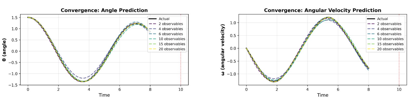
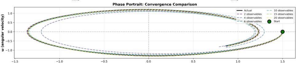
As you can see, the more variables we add, the closer we get to the actual behaviour of the pendulum! You can also see the improvement in phase space, where we plot the angle against the angular velocity.

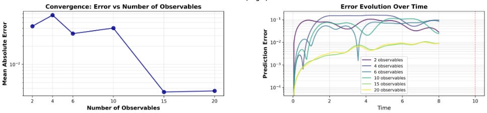
Taking the average of the errors, we can also see that the mean error decreases as we add observables.

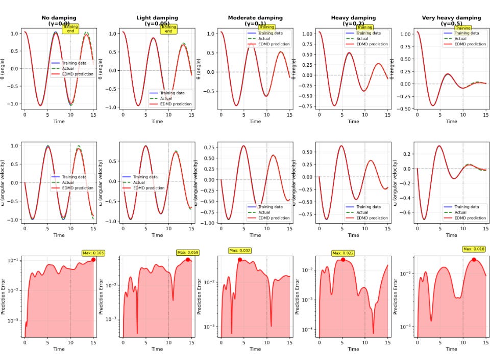
Ok, so how does this work for different levels of damping? Using six observables, we also find pretty decent results!

And so, I hope that you guys are convinced that there are some pretty cool methods to try and predict non-linear systems.

Thank you to David Jordan at Living Physics for the extensive discussions.

---

References

Koopman, B. O. (1931). “Hamiltonian systems and transformation in Hilbert space.” Proc. Natl. Acad. Sci. 17 315-318.