Computing a Feynman Diagram for the Magnetic g-Factor
Computing quantum level corrections to magnetic quantities in an electron.
A first look at the diagrams to compute the magnetic g-factor
In a previous post, I drew the diagram that gives the correction to our g-factor. It is a loop diagram — the photon connecting the electron momenta in the bottom creates a single closed loop, with momentum k. To compute the amplitude, we need to apply Feynman rules to this diagram. The diagram is daunting, but I’ll try to explain each element one by one.
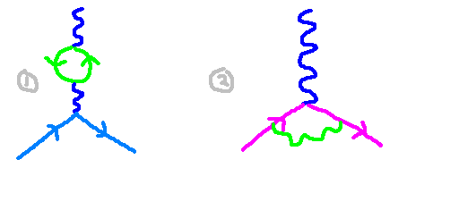
In the diagram above, we have an example of two different sub-processes used to compute the scattering of an electron with a photon. Next, we’ll try to understand how to calculate an explicit amplitude associated with the second diagram.
The Electron propagator
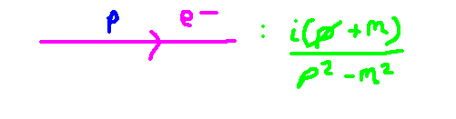
When we have an electron line in a diagram, we associate with it the propagator of an electron. A propagator represents the probability amplitude of an electron being generated at a point x ending at y. In the expression below, the spinor fields shown by the greek letter psi represent the electron in its initial and final state. The creation of the electron at x is represented by applying it to the ground state. This is why it’s squished up against the zero in the brackets. The ground state, by conventional notation, is represented by the zero in the angled brackets. This appearance of the electron at y is represented similarly by the spinor, whose argument is at y. The final propagator is then the contraction between these two states.

In the rightmost expression, the term in the integral is our propagator in momentum space. In the middle expression, the T represents a time ordering operator. Time ordering operators are a mathematical subtlety that is beyond the scope of this article. However, there are several steps needed to compute the integrand. First, spinors can be expanded out into smaller bits involving creation and annihilation operators. We expand the spinor at x and at y separately, which often creates a jumble of terms. We then mix these terms, and many of them simplify due to relationships between these creation and annihilation operators. It is then after this mess that we finally get the expression for the electron propagator.
The photon propagator
We do something very similar with the photon. The photon propagator is an amplitude that involves the vector potential A, instead of the spinors that we used for the electron propagator. Calculating this is quite similar to the process above, but there are easier ways that involve Fourier transforms. Again, there is a subtlety involved here. It turns out that there is a degree of ‘gauge freedom’ when defining what the propagator is, which arises from the symmetries in electromagnetic theory. This gauge freedom is represented by the Greek letter Xi in the expression below.

Computing the Diagram
Our diagram has three vertices. Vertices are the points where each line intersect — and they each contribute a scaling factor to our final amplitude. This scaling factor is our coupling constant. The more vertices a diagram has, the more negligible contribution it brings to the entire process. At each point ‘or vertex’ in the diagram, momentum needs to be conserved. This means that the sum of the momenta going into each vertex, must be the same as the sum going out.
There are three external legs in the diagram, which are lines that are not in between vertices. There are two electron external legs, and one photon external leg. For these external legs, we pre-define the momenta q_1, q_2 and p. We then try to compute the momenta of the internal lines (or propagators) with some simple arithmetic. After some playing around, it’s not too hard to convince yourself that due to the loop, there is one undetermined momentum which we will call k. I’ll explain what to do with this shortly.
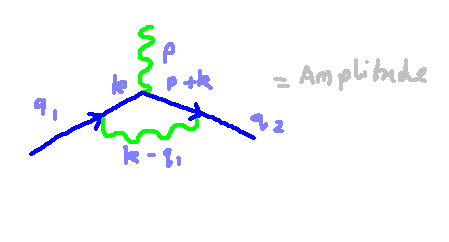
In addition to the external legs, we have three internal propagators. We have two electron propagators — one of these propagators uses the momentum k. The other propagator uses the momentum p+k. We also have an internal photon propagator with momentum k-q. All of these three momenta are shown in the above diagram. To get the total amplitude of these diagrams, we multiply each of these propagators together in one long expression. We then integrate over the free momentum k. The expression below is only a rough schematic of what the total amplitude looks like, but I think it gets the point across.

The exact mathematical expression is complex. You can see that in the denominator, there are three different factors. Each of these factors come from the denominator of the three separate propagators. The first factor contains a term that includes the (k-q_1)² term from the propagator associated with the photon. The other factors are functions of the momenta of the incoming and outgoing electron propagators. The numerator on the top of this fraction comes from the electron propagators and several intermediate terms that stem from the vertices.

Evaluating this expression is complicated. Very hard. Luckily, there are some tricks (like Feynman’s integral trick) that we can use to simplify things. I’ll elaborate on these tricks in the next section.
References
[1] Quantum Field Theory and the Standard Model by Schwartz, Matthew D. (ISBN: 8601406905047)