The Integer Quantum Hall Effect
Most of the time, we don't get to 'see' the results of quantum mechanics or general relativity coming out so obviously in an observation or an experiment. The phenomena are elusive is because the energy scales at which interesting phenomena occur are usua
A mysterious quantum story about magnets and electrons
Most of the time, we don't get to 'see' the results of quantum mechanics or general relativity coming out so obviously in an observation or an experiment. The phenomena are elusive is because the energy scales at which interesting phenomena occur are usually too small or too big to appreciate. So nature, to first order, is quite dull.
There are, however, some exceptions. For example, in general relativity, the Event Horizon Telescope took a picture of Messier 87's black hole. The photograph is an almost miraculous demonstration of the existence of spacetime singularities, infinite holes in the fabric of spacetime. In quantum mechanics, we have observed the band structure of hydrogen and the photoelectric effect — both experiments that reveal the 'discrete' nature of fields at the microscopic level.
There is a fantastic demonstration of the quantum nature of materials with the conductivity of metals under an applied magnetic field. These are called the quantum Hall effects. There are two different effects — an 'integer' effect and a 'fractional' effect. It is a peculiar phenomenon that involves a rich story of geometry, physics and experiment. I will talk about the integer effect in this post — what it is and how we can begin to explain it.
There is too much even to begin to explain the current state of research in just one article. So, I will describe the integer quantum Hall effect and then offer the first step to understanding its energy levels.
What is the Hall effect?
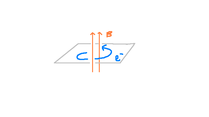
The original Hall effect was discovered in 1879 by Edwin Hall¹. Let's say you have a slab of two-dimensional metal lying face-down. Using an electric source, we can push a current through the metal. At the same time, using a magnet, we can push a magnetic field right through this plate. The diagram below shows the experiment. We can create the magnetic field by placing the north pole of a strong magnet above the metal slab and the south pole below it.

Now, what happens in this scenario? Well, if the magnetic field and the electric field are kept constant, it turns out that there is an induced electric field that moves across the slab, shown in the diagram below! The reason for this is interesting. Maxwell's equations predict that the electrons will start to bend when a magnetic field is applied — they curve. At average temperatures, electrons obey a model that is called the 'Drude model' of electromagnetism. The Drude model is an equation that governs how charged particles behave when under the influence of electromagnetic fields. The equation below shows the Drude model.
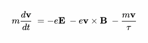
The first term on the left-hand side of the equation is an expression for the acceleration of a particle, and as you can see, it is a function of three different forces. The first factor involves the electric field E. This force moves the electron in the same direction as the magnetic field. The second force involves the magnetic field B. The cross in the expression means that the magnetic field will cause a twisting circular motion on the election. The final expression is the friction that an electron experiences bumping with other electrons in the material.
In this particular setup, with the electric and magnetic fields set up, the Drude model predicts bending in the anti-clockwise direction. This is shown in the dark blue arrows in the diagram below.

When the electrons curve and bend due to the Drude model, they begin to collect on the left side. Since it turns collectively on the left, it creates a collection of negative charges on the left side of the plate, which causes an induced electric field. This induced electric field is there because there is an imbalance of charge on the left side versus the right side of the plate. This induced electric field is shown in the light blue arrows and slowly gets stronger and stronger until the electrons travel in a straight line again, in the direction of field I. This result is called the Hall effect.
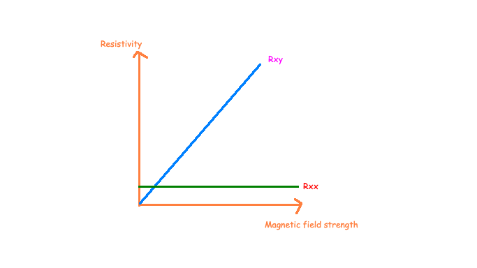
Now, for every metal, we have a measurable quantity called resistivity. Resistivity measures the difficulty of current flowing in response to an applied electric field. In the example above, we indeed have an applied electric field, and we can measure the resistance involved in inducing the current I. In this case, there are two types of resistivity.
The first type is called Rxx. This is the resistivity which looks at the resistance of the applied electric field's effect on current in the x-direction. This kind of resistivity is called longitudinal resistivity.
The second type is Rxy, the applied electric field's resistance effect on current in the y-direction. This type of resistivity is called Hall resistivity. Hall resistivity is linked with the induced electric field from the Hall effect discussed in the previous paragraph.
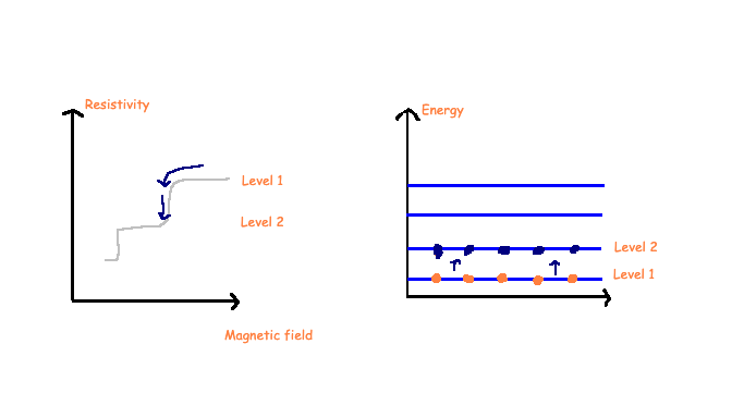
In the regular Drude model, there is a prediction on how the resistivity changes with the magnetic field's strength. To no surprise, the resistivity's relationship with the magnetic field is a boring one. For example, Rxy varies linearly with the size of the magnetic field, and Rxx remains constant. These relationships are shown in the diagrams below.
What happens at cold temperatures and when the magnetic field is large?
At average temperatures, we find that experimentally, this holds! As we ramp up the temperature, the Hall resistivity also increases linearly. However, something unusual happens when we dial up the strength of the magnetic field. When we dial up the strength of the magnetic field, we are no longer in the regime when the Drude model is valid. At this level, we see quantum effects start to take place, and it is simply astounding.
In experiments done in 1980 by von Kitzling, it turns out that the Hall resistivity no longer increases linearly. Instead, it appears that it grows in a step-wise fashion, plateauing and then increasing by an integer amount. A diagram of this baffling phenomenon is shown below. The longitudinal resistivity appears to be a straight line in the beginning and then evolves to look like single spikes at different values where the plateaus increase.
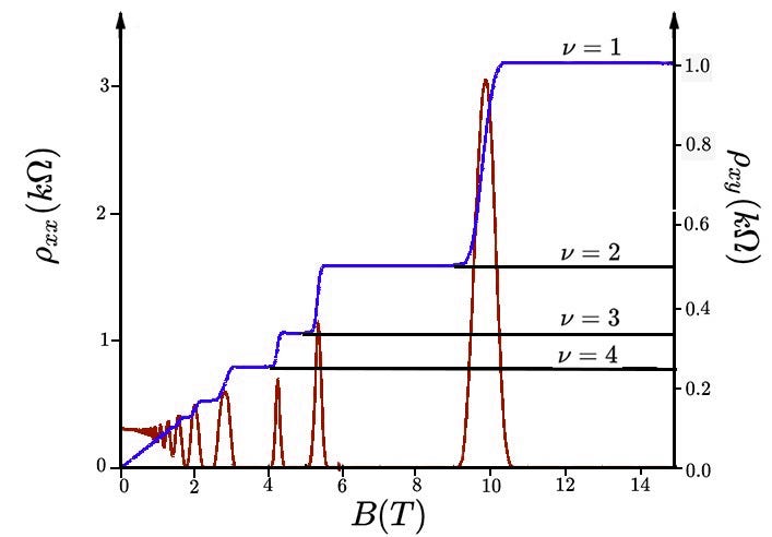
If you look close to the origin, we can see that the classical prediction by the Drude model holds. However, when we get to stronger magnetic fields, we start to see the weird 'jumping' of the Hall resistivity from level to level. The jumping is a quantum effect — discrete jumps like these ones are often associated with quantum phenomena.
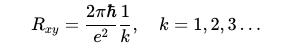
This is the integer quantum hall effect — it is called the integer quantum hall effect because the values of the plateaux lie at the values parametrised by integers k, shown below:
Landau Levels
So, we've seen above that the conductivity of the material jumps between discrete sets of values. Now, why does this happen? Well, it has to do with the quantum mechanics of a system — the mechanics of the electron force some of its physical properties to only be locked in specific discrete values. We need to understand the kinds of energy levels an electron can have when it's immersed in a magnetic field to understand this.
Just as a disclaimer — in the following section, I will not be going into great depth, but I hope to at least convey some basic dynamics that are going on.
When an electron is exposed to a magnetic field, a simple calculation using Maxwell's equations demonstrate that it orbits around in a circular fashion. This orbiting electron system will carry some energy. Classically, it could have any energy we want. However, in the quantum regime, it has been observed that the energies of this system can only take on discrete sets of values. These discrete states of energy, named after the Soviet physicist Lev Landau, are called Landau levels.
The mathematical justification for this is a little bit tricky, but I will do my best to explain it. To figure out the dynamics of a physical system, physicists construct the Hamiltonian, and then try to figure out the available energies that the Hamiltonian allows. In the case above, the Hamiltonian combines the momentum of the electron from its movement and the work it has done coupling itself to the magnetic field. The momentum is shown as p, and the magnetic and electric fields are encoded in the symbol A.

Now, to determine the allowable energies that this system can take, we use the Schrodinger equation. The Schrodinger equation is an equation that takes a Hamiltonian from a particular system and tells us what states and energies it is allowed to have. In quantum mechanics, these states and energies are called eigenstates and eigenvalues respectively.
Now, it turns out that this particular system is part of a class of Hamiltonians called 'quantum harmonic oscillators'. Quantum harmonic oscillators are the quantum mechanical equivalent of the Hamiltonian used to describe the dynamics of a spring. The difference is that, for the quantum mechanical version, we have to tweak the math to work in the assumption that position and momentum are not simultaneously observable. Amazingly, it turns out that a feature of a quantum harmonic oscillator is that it has discrete energy levels, much like the discrete modes of a vibrating string! This is at its core why Landau levels exist. The energy levels are shown here.

Now, at each of these energy levels, there is a 'maximum' number of electrons that can occupy that level. The reason why there is a maximum number of electrons is because of the Pauli exclusion principle. The Pauli exclusion principle is a principle that restricts two electrons from being in the same space at the same time, so there is a separation that needs to be enforced between them. Hence, this restricts the number of electrons that can fill a particular energy level. Think of this like floors in a hotel that become fully occupied, one by one, as we add in electrons to each floor.

Now, here is the crucial bit. For reasons which I will sweep under the rug, we only care about the filled levels of this electron hotel. If the hotel floors are only partially filled, like in level 2 above, we still consider our material to be in the state representing only one filled level. This is precisely the reason for our jumpy behaviour in the conductivity of a metal.
The maximum density of electrons required to fill a Landau level is a function of the magnetic field strength applied. For a single Landau level, we are only allowed a density of certain electrons. The Landau effect predicts that the number density of electrons required to fill one level is dependent on how strong the magnetic field is.
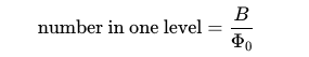
Because we said that only filled states matter, the number of electrons that a given material can have is locked at fixed multiples of how many electrons we can fit at one level. So, if we call the maximum number of states in one level k, then our number of electrons can only take values in the discrete numbers:

Now, let's link this back to the Hall resistivity. The Drude model says that the resistivity of a material depends on the number of electrons available in it. This fact seems to be true since the more electrons; the easier current flows through a material. However, this is precisely why our resistivity jumps between levels! Since we can only have a discrete set of electrons corresponding to our Landau levels, the resistivity shows the same pattern!
Wrap up
I hope that this article has given you a brief introduction to the quantum nature of magnets and resistivity! I have barely begun to scratch the surface and will probably go into more detail net time.
References
[1] Hall, EH. On a New Action of the Magnet on Electric Currents, 1879
[2] K. v Klitzing, G. Dorda, M. Pepper, "New Method for High-Accuracy Determination of the Fine- Structure Constant Based on Quantized Hall Resistance", Phys. Rev. Lett. 45 494.