Quantifying our Confidence in Statistical Models — The Confidence Interval
Newspapers try to inspire trust and credibility to their claims through the use of statistics. For the most part, it is often descriptive. Often, they are filler numbers, as newspapers need to convey that their articles are well researched. To this end, s
So you’re “90% sure” about something — what does that mean?
Newspapers try to inspire trust and credibility to their claims through the use of statistics. For the most part, it is often descriptive. Often, they are filler numbers, as newspapers need to convey that their articles are well researched. To this end, statistics are often included within the text.
A classic example of this is declarative statements about the stock market or some announcement by a governing body. I work full time as a trader for an American investment bank. In the office, headlines like ‘STOCKS RALLY 10% TODAY!’ or ‘FED CUTS RATES’ are constantly flashed on the TVs hanging above the trading floor.

These kinds of statements are either true or false and tend to be easily verifiable.
However, something that is not so obvious is when polls are involved. A poll is the use of a small sample to make a descriptive statement about a larger population. It is less evident in this case because there is some active inference used in a poll. Whilst a poll is easier to carry out, it doesn’t carry the whole picture. A vote doesn’t ask everyone. While this seems like an obvious objection and a clear counterargument to a poll, there are scientific ways to be sure. Sometimes, a vote can be helpful, and in other times, misleading. This article discusses the fascinating mathematics behind quantifying how certain you can be about a poll or any different estimate someone cooks up.
The art of deciding when a poll is ‘valid’ enough to have confidence in it is just as important as the data in the survey itself. We must be able to quantify a level of confidence in our beliefs about the world. Not only is it important to make quantitative conclusions about a state nature — it is also essential to quantify the uncertainty of those conclusions. Statisticians have a tool called the confidence interval, and I’ll write about it here.
Whilst I hope that newspapers nowadays aren’t so nefarious as to mislead the public actively, it would be wrong to say that they are without agendas. For example, a newspaper might have done a survey to assess how people feel about Joe Biden’s election. They might have done a study about how much fruit they eat on average. It could be anything, and it could force readers into believing a statement that is not reflective of reality. Hopefully, this article offers some colour on how we can decide when enough evidence is enough.
Probability Distributions
Inferential statistics is the art of modelling some real-life process or population with math to predict likely outcomes in the future. Most importantly, it involves using sampling to both inspire and verify the correctness of mathematical models. A sample is a small ‘snapshot’ of the entire population, and it is used to draw conclusions about the population as the whole itself.
The reason why we use samples is two-fold. Firstly, it is often too complicated or costly to survey every member of the population. Secondly, there are also instances where it is philosophically impossible to do so — for example, what if the act of observing an object destroys it? So, we need to create mathematical models with limited samples we have to make conclusions.
To do this, statisticians model a with probability distributions. Probability is just another word for describing how often you’d expect to see an event occur if the experimenter ran the same experiment multiple times. A probability distribution is a function that assigns a chance to some event happening. It is called a distribution since the probabilities assigned to different events are ‘spread out’ across different outcomes. Let’s take a coin as an example. It lands half of the time as heads and half of the time as tails. The probability of 0.5 is assigned to each side of the coin. Mathematicians and statisticians call this a binomial distribution. The ‘bi-’ comes from the fact that there are only two outcomes.
In this case, the parameter of the binomial distribution is p=0.5 since the probability of heads is 0.5. A parameter(s) is a number(s) that characterise a probability distribution somehow. If the coin was biased tilted towards heads, say 60%, then p=0.6.
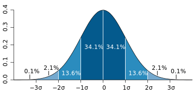
Let’s take another example — the heights of a population. In this case, we expect that people on the extremely tall or short ends of the distribution are less prevalent in a population. The name for the distribution that is used to commonly model height is somewhat oddly called the ‘normal’ distribution. There are countless different distributions that mathematicians have cooked up to describe various phenomena. They all have other esoteric names like the ‘gamma distribution’ or the ‘beta distribution’. Whilst they are engaging in their own right, I’ll be looking at examples from the binomial and normal distributions to start.
Estimates from a distribution
The usual dance in the ‘frequentist’ method of statistics is this. We first have a population that we’d like to model. We then need to decide which distribution is the best to use to model it. There are two questions to ask here — what type of distribution is it? What are the parameters of the distribution? There is an art to picking the kind of distribution. Say we wanted to model people’s weights in Europe — we could use a normal distribution, a Chi-squared distribution, a Poisson distribution, who knows? Once we have done that, we then have to find the associated parameters.
For example, in the normal distribution, we have two parameters. The mean is the most common number to pop out of the distribution, and the standard deviation. The statistician’s job is to find ways to determine then what these parameters are.
Let’s say we have good reason to believe that the mean heights are normally distributed. Now, all that’s left to do is determine the parameters — the mean and the standard deviation. Since measuring every single person would be too taxing, we take a sample. For example, suppose we take a sample of 10 people taken from this Earth’s population of 7 billion people. Then, our estimated mean would be the arithmetic mean of the heights of those ten people.
Similarly, the standard deviation can also be calculated from a sample. The calculation looks at the distances the data are from the mean of the population. However, since these are merely calculations taken from a sample, there are questions about their validity. The dodginess begs the question, how sure are we about the estimates of these parameters? Intuitively, you would put your faith in an estimate which was measured from more people as opposed to less — is there a mathematical way to quantify this level of confidence?
The simplest example
A standard tool in the statistician’s toolset is to use confidence intervals to answer the question above. A confidence interval captures a degree of accuracy in our sample estimates. We commonly see the use of confidence intervals in statistical literature and data journalism. Once calculating a confidence interval — say the average weight of an apple, many would then say (including the general media) something along the lines of
‘we are 95% sure that apples on average lie in between 490g and 510g’
The procedure to calculate a confidence interval is tricky and mathematically fiddly. Nevertheless, confidence intervals convey some degree of certainty around an estimated quantity taken from a population sample. In the frequentist approach to statistics, we assume that some parameter in nature has a true fixed value — and our job is to ‘estimate’ that fixed value. I will describe how confidence intervals are constructed, then try to unpack their meaning and shed some light on why the above quote is murky.
To construct a confidence interval, mathematicians combine the estimates into a form that they understand. First, the estimates themselves have a distribution. Then, with some mathematical trickery, we massage them into a formula like the one below. For example, in the case of the normal distribution, if we want to compute a 95% confidence interval, we substitute the values of our estimates into the following expression.

In the above, s and n are the sampling standard deviation and sample size, respectively. The greek letter μ is the estimated mean we calculated earlier. Finally, we set z=1.96 to build a 95% confidence interval.
Now, on to the main point of the article. What does this mean exactly? I see confidence intervals used all the time in scientific journals and the media, but it’s hard to interpret what they mean. The common thought is that this is the probability that the true value is contained in the interval. Now — is this even correct the correct interpretation for the usual calculation? It can’t be — there is no such thing as a probability distribution for something true and fixed. It is slightly more subtle than this, depending on your philosophical leanings. The interpretation and true meaning was quite a difficult thing for me to grasp.
The way to square this philosophical fiddling is to slightly modify our interpretation and reframe it in terms of repeated experimentation. For example, suppose I estimate the mean with some procedure and come up with two bounds (90, 110) as some 95% confidence interval. In that case, this is not the probability that the actual value lies in the confidence interval.
Instead, we reframe this to the following interpretation. We are ‘95% sure the confidence interval contains the true value’. This sentence means that if we were to repeat the same procedure of constructing this interval 100 times, we would build an interval that contains the true value 95% of the time. Hence, the excellent definition of a 95% confidence interval is — ‘if a were to repeat the same sampling procedure 100 times and construct a confidence interval each time, then I expect that 95 times the confidence interval should capture the true value’.
A footnote: What does it mean to say am x% sure about something?
People often say that they are “60% sure” or “70% sure” that something will happen in less intense contexts. For example, if I am 80% confident that I am right, what does that mean? Let’s take a more straightforward case. For instance, if I am 50% sure that the next coin flip would turn up heads, what does this mean? Does this equate to me saying that there’s a 50% chance that it will? Declaring the probability that something happens is not necessarily the same as being ‘sure’ that it will happen.
I propose that the most sensible interpretation of the above statement here. Imagine that we are savant stock analysts. We are asked how sure we are that a company was going to go bankrupt. If I said we were 20% sure, it means that I would choose to play ‘the game’ in the following set-up:
Suppose we are given a choice to either
play a game, or,
bet on the company going bankrupt.
If you choose to play the game, the game is simple — you win a million dollars if you select a green ball from a bag with 20 green balls and 80 red balls. If you choose to bet on the company going bankrupt, you win a million dollars if it does.
We are at most 20% sure that it will go bankrupt if we’d rather win a million dollars from selecting from the bag than choosing to bet on the company.
There’s an excellent article here on the semantics behind how different words equate to different perceived probabilities.
Wrap up
I hope that this article has shed some light on how statistics can be used to determine confidence in a poll. I am not a statistician, but thinking about things in terms of probability distributions helps me make confident conclusions about nature.
References
[1] Casella Berger, Statistical Inference, 1990