Non Equilibrium Statistical Mechanics and Biology
A cool type of math suited to some biology problems.
In high school physics, we tend to consider systems with ‘easy’ assumptions. They are deterministic systems, in a vacuum, and in equilibrium. In classical mechanics, this means that one uses the techniques of Newton; I consider a particle in a vacuum, cleanly calculate the forces on it, balance the forces out, then get the quantities I desire. Thermal Equilibrium means that the system we consider doesn’t transfer energy out into its environment. This works for most things at normal energy scales!
However, in biology, even though we are working with normal energy scales, these clean assumptions don’t hold. We study systems in fluids like water, which is composed of many moving molecules interacting with the system. This complicates the math since there is friction on the macro scale, and thermal fluctuations (water molecules are continually bumping against the system even when its at ‘rest’). They really are same sides of the same coin, but I’ll explain this later.
My main point is that in biology, its necessary to use different tools. This week I’ve learnt that biological problems are particularly suited to a field of math called non-equilibrium statistical dynamics, which studies the macro dynamics of systems under microscopic random forces, and for which there are energy imbalances.
For the rest of this post, I’m going to describe a toy model on where these random forces play a role.
Let’s take the example of a particle moving due to friction through a fluid. Let’s call this friction coefficient ξ - we will need this for later.
In the diagram below, the left hand side shows the classical case. If we give the particle some initial speed, the friction will cause it to slow down. Classically, in a fluid, this is known as Stokes law. The friction term is negatively proportional to the direction at which the particle is moving, which causes it to be at rest after some time.
But now consider the case on the right hand side, where we model the particle as moving in a bath of water. After giving it some initial speed, we still expect the particle to obey friction in the macro sense as it moves through the fluid. But the difference is, after a long period of time, we don’t expect to be at rest. It is kind of at rest, in the sense that on average its velocity is zero, but still jiggling about due to all of the random knocks of the water molecules. So, we need to we add the random, small scale interactions of the water molecules to the particle, modify our equation, and write this in a term, delta F, on the right hand side. This term is random, obeys some distribution with zero average direction, but has some strength, and is called a thermal term.
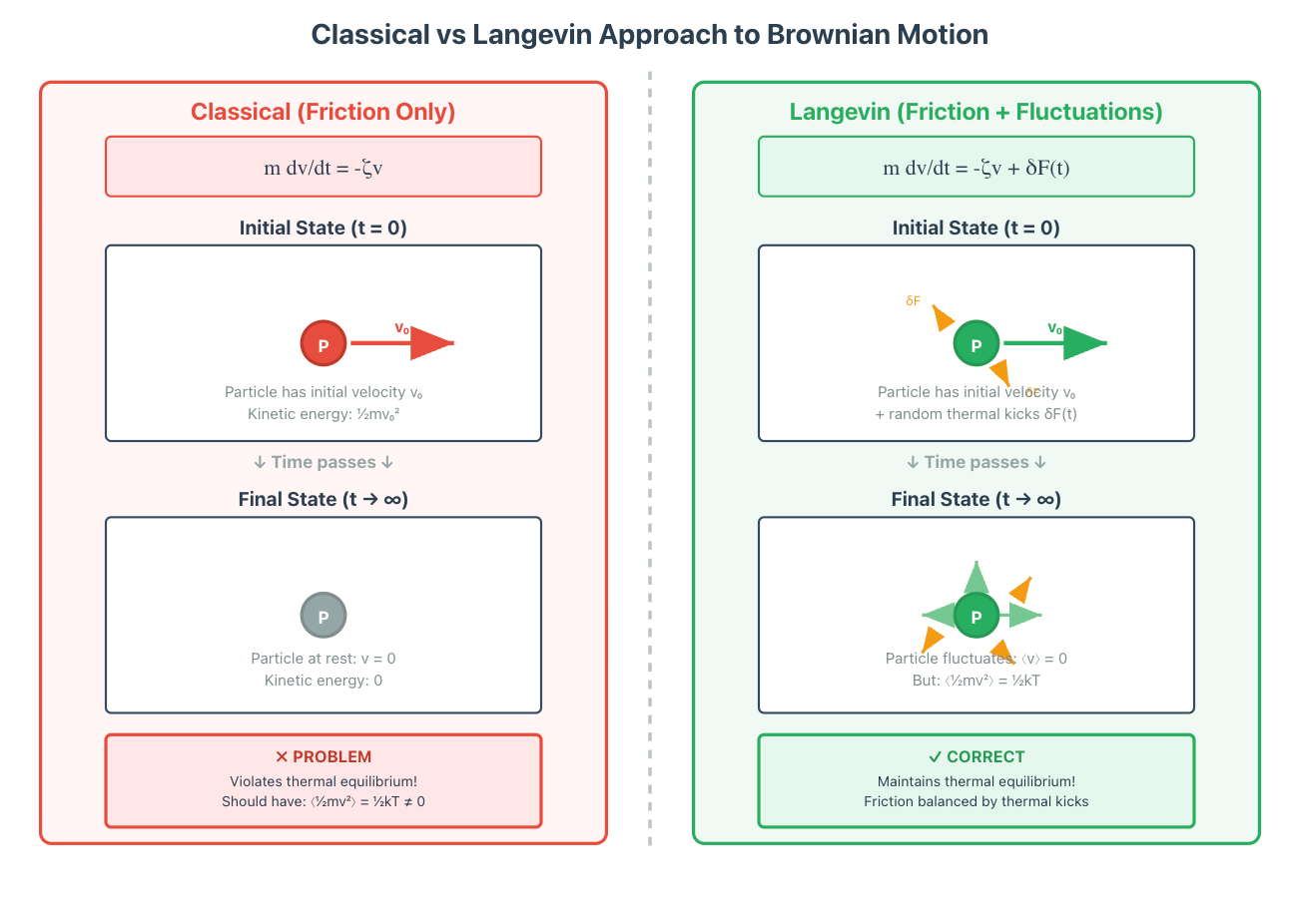
Once you add this term, you get something called a Langevin equation. When you solve the equation, what happens is that the friction term dominates initially, slows the particle down, and then makes it settle in a state where on average it doesn’t move. But, its always jiggling around with some energy that matches the thermal background around it.
So what’s the catch? Where is the math useful? Well, this is where we can find some cool and deep results.
If we define the fluctuation term delta F to depend on some arbitrary parameter B, then after some math [Zwanzig, 2001], we find that we can actually relate this fluctuation strength to the friction coefficient ξ itself, where k is the Boltzmann constant, and T is the temperature.
This is really deep. Its called a Fluctuation and Dissipation Theorem (of which there are many types), and it relates the size of the thermal fluctuations B to the friction. Intuitively, this makes sense, because what is friction if not just micro molecules bumping against us? And so, if the strength of the fluctuations increased, violently bumping up against the particle, so would the friction.
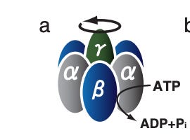
How is this useful? Well, non-equilbrium stat mech uses these sorts of setups to relate energy effects, which are hard to measure in systems where thermal fluctuations are dominant, to experimentally observable quantities. For example in Toyabe et al (2010) they used a result by Harada and Sasa to estimate the energy efficiency of a molecular motor called F₁-ATPase. Traditionally, this would’ve been hard since its impossible to measure the heat dissipation of such a molecule in a water bath. But with non-equilibium stat mech, they were able to relate it to experimentally observable quantities of a probe they attached. Pretty sweet!
References
Zwanzig, R. (2001). Nonequilibrium Statistical Mechanics. Oxford University Press, New York.
Toyabe, S., Okamoto, T., Watanabe-Nakayama, T., Taketani, H., Kudo, S. & Muneyuki, E. Nonequilibrium energetics of a single F₁-ATPase molecule. Phys. Rev. Lett. 104, 198103 (2010).
Wow, super interesting.