How do Loops change Physics?
An Example of Renormalisation in a Simple Scattering Problem
In previous frameworks of field theory, obtaining quantities of interest often lead to infinities in the calculations. For example, consider the problem of two massless particles scattering off one another. The mechanics of this scattering problem is described by a theory that has certain parameters that we might wish to measure. The suppose that the only parameter that described this theory was some interaction term lambda. It can be shown with the earlier techniques of quantum field theory that calculating the probability amplitude of this scattering problem is infinite! I will show this calculation in the next section.
$$ \text{Initial value of } \lambda \implies \text{divergent value of scattering probablity } \implies \text{fix } \lambda $$
So, we’ve arrived at a physical quantity that seems impossible. This is obviously is nuts - so how would we rectify this issue? The logical conclusion is that the initial value of lambda that we postulated in the beginning mustn’t be finite. In fact, it must be formally infinite, and when the contributions from loops in field theory are added, the must work to cancel out this infinity to arrive at quantities that are finite and observable. So, we have to find a way to circumvent these infinite constants with some mathematical machinery.
“Bare quantities” are the quantities you get from studying a quantity of interest, and then adding loop contributions into the mix. For example, the calculation of the bare mass of an electron is formally infinite in quantum electrodynamics. To see this, we can study loop contributions from the electron propagator. In addition, the calculation of the bare charge of an electron is also infinite. This can be seen by looking at loop contributions to the photon propagator.
$$ \begin{aligned} e & \iff \text{Photon Propagator} \\ m _ e & \iff \text{Electron propagator} \end{aligned} $$
These infinities come from the loop contributions in our integral, that are a result of high momentum, short wave-length phenomena. To tackle these infinities, In this post, I hope to outline simple examples of how renormalisation updates our view of the physical world, and modifies the physical laws around us. I think this viewpoint of seeing how simple examples change is useful since many of the textbooks I’ve read don’t seem to make specific references to how developments in quantum field theory have refined our physical modelling of the world.
The example about a simple scattering problem
We’ll start from scratch with a simple, scalar theory. Recall that scalar fields are fields that just assign a single number to different points in space-time. This kind of theory would be relevant to bosonic particles - not particles like electrons. Suppose we have a theory that describes a field with mass, but with a single interactions term given by a phi-four term. What are the quantities of interest? Well, the interaction term lambda would be the easiest place to start exploring some interesting questions.
Let’s try figure out the things we can learn from this field. Namely, what does scattering look-like, and how does the first order approximation change when we include loop contributions? In the section below, we will be calculating how cross sections change depending on the energy of the collisions, and how this view changes with renormalisation. Let’s start with the simplest Lagrangian we can think of, which is a massless field with some self interaction term.
$$ L = \frac{ 1 } { 2 } (\partial_ \mu \phi ^ \mu \partial \phi ) + \frac{ \lambda}{ 4!} \phi ^ 4 $$
One of the first things we can do is calculate scattering amplitudes. More specifically, we will be taking a look at the simplest thing to calculate - what is the cross section of two of these particles scattering off of each other? The input probabilities in this case will be p1, p2, and the outgoing probabilites will be p3 and p4. To calculate a cross section, we can use Feynman rules for different diagrams and then count. So, at tree level, we have that the amplitude is given by the following diagram.
$$ M_{\text{tree}} = - i \lambda $$
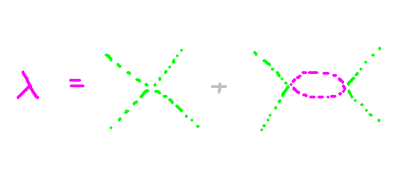
This is already interesting, it tells us that the amplitude is not a function of the inner or outer momentum! Now, what happens when we include loop contributions? Loop contributions are diagrams that contain the same input and output scattering processes, yet have loops in the diagrams embedded within them. We have contributions from loops, and this gives us another contribution to the scattering probability. The loop is shown in the diagram above, on the right. I will not put the loop calculation here, but just quote the result instead. The loop integral is divergent, so we cut it off at the value Lambda. The capital Lambda here is some artificially imposed cut-off that we use to contain the divergences from the infinite loop contribution. In the limit, Lambda here goes to infinity.
$$ M_{\text{loop}} = - \frac{ \lambda ^ 2 } { 32 \pi ^ 2 } \ln \frac{s} { \Lambda ^ 2 } , \quad s = p ^ 2 $$
The total amplitude here is the sum of the tree contribution and the loop contribution. Now, suppose that we measured the value of lambda in an experiment. This would mean that our value of lambda that we observe is equal to the tree level contribution, as well as higher loop contributions. This means that we have the expression below.
$$ \lambda _ R = \lambda + \frac{ \lambda ^ 2 } { 32 \pi ^ 2 } \ln \frac{ s } { \Lambda ^ 2 } - O ( \lambda ^ 3) $$
This is already interesting. The original sum of contributions from the theory was infinite, so we resolved this problem by enforcing a finite cut-off. The sum however, of the two terms, is finite, which implies that the original Lambda must be an infinite quantity. In physics, we want to come up with a model that predicts what happens when we repeat the experiment at a different energy. So, let’s try compute the scattering amplitude at a different energy level, s’.
$$ M ( s ' ) = - \lambda - \frac{ \lambda ^ 2 } { 32 \pi ^ 2 } \ln \frac{ s' } { \Lambda ^ 2 } - O ( \lambda ^ 3) = - \lambda _ R - \frac{ \lambda _ R ^ 2 } { 32 \pi ^ 2 } \ln \frac{ s' } { s} - O ( \lambda ^ 3 ) $$
So, the new scattering amplitude is indeed a function of our first measurement, lambda_R. However, the amplitude is indeed a function that varies with the energy of the new scattering set-up relative to the energy of the old scattering set-up! Had we considered just tree level contributions, we would have not found this relationship.