A Quantum Mechanics Problem on a Particle in a Line under an Electric Field.
Quick exercises inspired by hard problems.
Here are some problems very loosely inspired by a few months’ work looking at graphene band structure. In particular, I tried a bunch of computational methods to compute the band structure of graphene under electric fields, but it didn’t work since it’s so hard to get the compute set up. In fact, I plan to write another post on how unreasonably difficult it is to set this up for newcomers in the field.
So, the computational method is a bust for now, but this got me thinking - how far can we go with just analytical solutions to figure out some of the tricker properties of graphene? In particular, the problem we are looking at is what happens when we put some idealised graphene structure in water or expose graphene to electric fields. This gives some neat problems
You have a system where an electron can hop between two atoms - what are the energy levels allowed in this system?
Suppose you have an infinite line of atoms, and you place a dipole at the top - does this construction still have a band structure? you would think not, since its no longer periodic. But, you could have an array of dipoles with a different frequency at the top to make it periodic. This is quite an interesting problem.
How would you add an electric field to an electron? The electron feels a force due to the Lorentz force. This should be a potential, and this potential causes some motion change.
The Case of a Particle on a Finite Line with an Electric Field
(Side note: I’m surprised there aren’t more expositions about this problem in university courses, but maybe it’s because we have to deal with Airy functions).
To warm up, let’s what are the possible energy levels of an electron trapped on a finite line, under the influence of some external electric field. This starting exercise is useful because it is a boiled-down toy model of the problems above, and it’s in one dimension. To work quantum mechanically, we need to solve Schodinger’s equation. Schrodinger’s equation tells us what the wavefunction and the possible energy levels are, given some Hamiltonian. In quantum theory, it proposes that the wavefunction should merely be scaled under the influence of a Hamiltonian and that these wavefunctions are precisely the physically allowed states. The scaling factors, furthermore, are the permitted energies.
The Hamiltonian is the sum of the kinetic energy of the wavefunction and the potential energy. The expression for the kinetic energy of a wave function is known, and we call it T. For the purposes of this exercise, I am setting Planck’s constant to 1, just so we see the math that comes out.
So, what’s the potential term? We know that by the Lorenz force law, the force felt on an electron with a charge q should be equal to the electric field vector multiplied by that charge. As a reminder that this is true, you can convince yourself by trying to guess the motion of what happens when you put an electron between a positive and negative terminal (the electron would float towards the positive terminal by the law of attraction.
From basic mechanics, we know that the force is equal to the grad operator of the potential, and hence, if the electric field is uniform, we can guess the form of the potential that will give us this field.
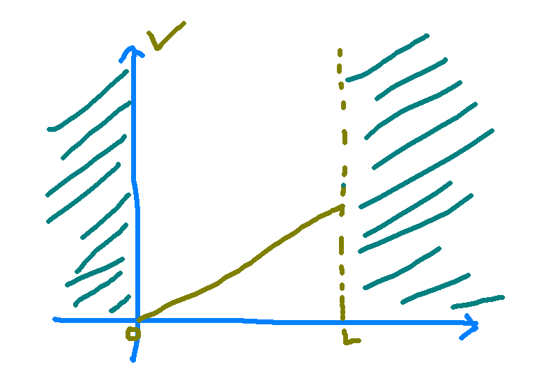
This is great! We now have solved what the potential looks like and can now plug it into Schrodinger’s equation and try to solve that equation. The potential is a linear potential, and so our setting looks like this where we set the regions outside the line L to an infinitely high potential to make sure that the electron can’t go there.
If we take the sum of the potential term and the kinetic term, we get the neat equation below, and our mission now is to solve for phi, the save function.
At this point, we have to answer two mathematical questions. Do solutions exist, and if so, with the boundary conditions - what does this look like? It turns out this is not really an equation you can solve with just some elementary methods. After some math, we find that this looks like a linear combination of Airy functions, the solution to this is given by the following, referenced here. https://theory.physics.manchester.ac.uk/~judith/AQMI/PHYS30201se31.xhtml
These Airy functions are precisely the solutions to the simpler form, so to get this solution, you can reduce the earlier equation into simpler variables and then substitute it back out.
Now, what do these solutions look like? Well, let’s examine the extreme case where we set the potential V = 0. We know that the solution to a particle in a box, without any potential, looks like waves whose frequency increments by integer numbers. So, we would expect that for small values of V, that the Airy functions look ‘wavelike’ to some degree. And this is exactly the case!
The constants C and D are determined by boundary conditions, which are the values of the wave function for which we already know the values. For a line of size L, we should expect that the probability distribution at the ends of this line go to zero. All of the other constants in the brackets are some function of the constants m, q, and E, but as we’ll see later, we don’t actually need to know what those values are. If our line is bounded such that
Substituting it to solve for C and D in the equation above necessarily forces our wave function to be zero everywhere, so for the problem above, we get that there are no solutions to Schrodinger’s equation.